Machine Learning, Python, Artificial Intelligence
Build a Movie Recommendation System in Python

A movie recommendation system predicts which films a user will enjoy and ranks them for that person. Netflix, Prime Video, and Letterboxd all run on this idea, and you can build a working version in Python with pandas, scikit-learn, and the MovieLens dataset in a single afternoon. This guide walks the full project: the three recommender types, the code for each, how to evaluate them, and how to serve the result behind a Flask API. If you get stuck on a graded version of this, our machine learning assignment help team builds these end to end, and you pay half upfront and half after the code runs on your data.
What a recommendation system actually does
A recommendation system maps a user to a ranked list of items they have not seen yet. The input is interaction data, usually ratings or watch history; the output is an ordered list of movies, best match first. Three families dominate the field, and each answers a different question.
| Recommender type | Core question | Needs | Strength | Weakness |
|---|---|---|---|---|
| Content-based | “What looks like what you already liked?” | Item features (genre, cast, plot) | Works for brand-new movies | Stays inside one taste bubble |
| Collaborative filtering | “What did similar users like?” | A user-item ratings matrix | Finds taste it cannot describe | Cold start for new users and items |
| Hybrid | Both, combined | Features and ratings | Covers each method’s blind spot | More code to maintain |
The project below builds all three so you can compare them on the same data. Recommendation differs from box office prediction, which is a regression task that forecasts revenue. Here the goal is ranking, and the metrics reward putting the right films near the top of the list.
Set up the project and environment
Start with an isolated virtual environment and a clean folder layout so the data, notebooks, and source code stay separate. This keeps dependency versions pinned to the assignment brief and makes the project reproducible on a grader’s machine.
python -m venv movie_rec_env
source movie_rec_env/bin/activate        # macOS or Linux
# movie_rec_env\Scripts\activate         # Windows
pip install pandas numpy scikit-learn scikit-surprise matplotlib seaborn flask
Pin the versions in a requirements.txt so the grader installs exactly what you tested against:
pandas==2.2.2
numpy==1.26.4
scikit-learn==1.4.2
scikit-surprise==1.1.4
matplotlib==3.8.4
seaborn==0.13.2
flask==3.0.3
A predictable folder structure separates concerns and reads well in a repository:
movie_recommender/
├── data/
│   ├── raw/                 # MovieLens and TMDb CSV files
│   └── processed/           # cleaned, merged tables
├── notebooks/
│   ├── 01_eda.ipynb
│   └── 02_modeling.ipynb
├── src/
│   ├── content_based.py
│   ├── collaborative.py
│   ├── hybrid.py
│   └── evaluate.py
├── app.py                   # Flask serving layer
├── requirements.txt
└── README.md
Get the data: MovieLens and TMDb
Two datasets cover every recommender in this project, and both are free. The choice between them depends on which filtering method you are feeding.
- MovieLens 100K from GroupLens holds 100,000 ratings from 943 users across 1,682 movies. The ratings matrix is exactly what collaborative filtering needs, and the dataset is small enough to load into memory and iterate on fast.
- MovieLens 25M scales the same format to 25 million ratings once your pipeline runs and you want a realistic benchmark.
- TMDb 5000 Movie Dataset adds plot overviews, genres, keywords, cast, and crew. Content-based filtering reads these text and category features, so this is the table that powers similarity by item attributes.
Load the MovieLens ratings and the movie titles, then merge them on the movie id:
import pandas as pd

ratings = pd.read_csv("data/raw/u.data", sep="\t",
                      names=["user_id", "movie_id", "rating", "timestamp"])
movies = pd.read_csv("data/raw/u.item", sep="|", encoding="latin-1",
                     usecols=[0, 1], names=["movie_id", "title"])

data = ratings.merge(movies, on="movie_id")
print(data.shape)          # (100000, 5)
print(data["rating"].describe())
To pull richer metadata for content-based filtering, the TMDb API returns plot, genre, and cast as JSON. Store your key in an environment variable rather than the source file so it never lands in version control:
import os
from tmdbv3api import TMDb, Movie

tmdb = TMDb()
tmdb.api_key = os.environ["TMDB_API_KEY"]   # never hardcode the key

movie = Movie()
details = movie.details(550)                 # Fight Club
print(details.title, details.genres)
Save raw downloads to data/raw/ and write cleaned tables to data/processed/. Inspect every file for missing titles and duplicate movie ids before modeling.
Explore the data before modeling
Exploratory data analysis tells you what the model can and cannot learn. Three checks matter most for a recommender, and each one shapes a later decision.
First, look at the rating distribution. MovieLens ratings cluster around 3 and 4 on a 1-to-5 scale, which means a model that predicts “4 for everything” already scores reasonably on error metrics. That baseline is the bar your real model must clear.
import seaborn as sns
import matplotlib.pyplot as plt

sns.histplot(data["rating"], bins=5)
plt.title("Rating distribution")
plt.show()
Second, measure sparsity. With 943 users and 1,682 movies there are about 1.59 million possible cells, but only 100,000 are filled, so roughly 94% of the matrix is empty. High sparsity is the central challenge of collaborative filtering and the reason matrix factorization beats naive averaging.
n_users = data["user_id"].nunique()
n_movies = data["movie_id"].nunique()
sparsity = 1 - len(data) / (n_users * n_movies)
print(f"Matrix is {sparsity:.1%} empty")
Third, check the long tail of popularity. A small set of blockbusters collects most of the ratings while thousands of films get a handful each. A counter of ratings per movie exposes this, and it explains why a popularity baseline keeps recommending the same ten films to everyone.
Method 1: content-based filtering
Content-based filtering recommends movies whose features resemble a film the user already rated highly. The pipeline turns each movie’s text features into a numeric vector with TF-IDF, then ranks other movies by cosine similarity to the target. This method needs no other users, so it handles a brand-new title the moment its metadata exists.
Build one text field per movie from genres, keywords, and cast, then vectorize it:
from sklearn.feature_extraction.text import TfidfVectorizer
from sklearn.metrics.pairwise import cosine_similarity

# tmdb_movies has a "tags" column joining genres + keywords + cast
tfidf = TfidfVectorizer(stop_words="english", max_features=5000)
tfidf_matrix = tfidf.fit_transform(tmdb_movies["tags"])

similarity = cosine_similarity(tfidf_matrix)
Cosine similarity scores every pair of movies from 0 (unrelated) to 1 (identical direction). To recommend, find the target film’s row, sort the scores, and return the top matches:
def recommend_similar(title, movies_df, sim_matrix, k=5):
    idx = movies_df.index[movies_df["title"] == title][0]
    scores = list(enumerate(sim_matrix[idx]))
    scores = sorted(scores, key=lambda x: x[1], reverse=True)[1:k + 1]
    return movies_df.iloc[[i for i, _ in scores]]["title"].tolist()

print(recommend_similar("The Dark Knight", tmdb_movies, similarity))
The weakness shows up fast: content-based filtering keeps the user inside one taste bubble. A reader who liked one action film gets only more action films, never the comedy they would also enjoy. Collaborative filtering fixes that.
Method 2: collaborative filtering
Collaborative filtering predicts a user’s rating for a movie by learning from every other user’s ratings, with no item features at all. The strongest practical approach is matrix factorization with SVD, which splits the sparse user-item matrix into compact user and movie factor matrices. Each latent factor captures a taste dimension the model discovers on its own, such as a lean toward dark thrillers or feel-good musicals.
The scikit-surprise library implements SVD with a clean train and predict API:
from surprise import Dataset, Reader, SVD
from surprise.model_selection import train_test_split
from surprise import accuracy

reader = Reader(rating_scale=(1, 5))
ds = Dataset.load_from_df(data[["user_id", "movie_id", "rating"]], reader)
trainset, testset = train_test_split(ds, test_size=0.2, random_state=42)

model = SVD(n_factors=100, n_epochs=20, lr_all=0.005, reg_all=0.02)
model.fit(trainset)

predictions = model.test(testset)
print("RMSE:", accuracy.rmse(predictions))
To produce a top-N list for one user, predict the rating for every movie that user has not seen, then sort:
def top_n_for_user(user_id, model, all_movie_ids, seen, n=10):
    unseen = [m for m in all_movie_ids if m not in seen]
    preds = [(m, model.predict(user_id, m).est) for m in unseen]
    preds.sort(key=lambda x: x[1], reverse=True)
    return preds[:n]
Collaborative filtering captures taste that no feature list can describe, but it breaks on the cold start problem. A new user with zero ratings gives the model nothing to learn from, and a freshly added movie has no interactions to match against.
Method 3: the hybrid model
A hybrid model combines content-based and collaborative filtering so each method covers the other’s blind spot. The cleanest design is a weighted blend: score candidates with both methods, normalize each score, and combine them. When the user is new, the weight shifts toward content-based and popularity; once they accumulate ratings, the collaborative weight rises.
def hybrid_score(user_id, movie_id, cb_score, cf_model, alpha=0.5):
    # alpha balances content-based (cb) against collaborative (cf)
    cf_score = cf_model.predict(user_id, movie_id).est / 5.0   # scale to 0..1
    return alpha * cb_score + (1 - alpha) * cf_score
For a new user, set alpha near 1.0 so content and popularity drive the list, then lower it as ratings arrive. This single switch is how production systems handle cold start without a separate code path. The hybrid carries more code than either method alone, which is the trade you accept for coverage across new users, new movies, and established viewers.
Evaluate the recommender
The metric you pick depends on what the model outputs. Pick the wrong one and a graded assignment loses marks even when the code is correct.
| Output | Metric | What it measures |
|---|---|---|
| Predicted star rating | RMSE, MAE | Distance between predicted and real ratings |
| Ranked top-N list | Precision@K, Recall@K | Share of relevant movies in the top K |
| Ranked top-N list | NDCG@K | Relevance weighted by position in the list |
RMSE penalizes large misses more than MAE because it squares the error, which is why rating-prediction tasks usually report it. For the top-N list, Precision@K answers “of the 10 movies I recommended, how many were relevant,” while Recall@K answers “of all the movies the user would have liked, how many did I surface.” Compute Precision@K from the SVD predictions:
def precision_at_k(predictions, k=10, threshold=3.5):
    from collections import defaultdict
    user_est_true = defaultdict(list)
    for uid, _, true_r, est, _ in predictions:
        user_est_true[uid].append((est, true_r))

    precisions = []
    for uid, ratings in user_est_true.items():
        ratings.sort(key=lambda x: x[0], reverse=True)
        top_k = ratings[:k]
        n_rel_and_rec = sum(1 for est, true_r in top_k if true_r >= threshold)
        precisions.append(n_rel_and_rec / k)
    return sum(precisions) / len(precisions)

print("Precision@10:", precision_at_k(predictions, k=10))
Always compare against two baselines: predict the global average rating, and recommend the most popular movies. A model that cannot beat “recommend the top ten most-rated films” has learned nothing useful. This baseline comparison is the single check that separates a passing project from a guessed one, and many students skip it. If you want a second set of eyes on the evaluation before you submit, our machine learning assignment help developers test the metrics against the grader’s expected format and send back sample defense questions with the delivery.
Improve accuracy
Once the baseline pipeline runs, four levers raise quality without rewriting the approach.
- Tune SVD hyperparameters. The factor count
n_factors, learning ratelr_all, and regularizationreg_allchange accuracy noticeably. RunGridSearchCVfrom Surprise across a small grid and keep the lowest-RMSE configuration. - Add implicit signals. Watch time, clicks, and add-to-list events carry taste even when the user never leaves a star rating. Treating these as weak positive signals densifies the matrix.
- Regularize content vectors. Cap
max_featuresin TF-IDF and drop rare keywords so the similarity scores key off meaningful tokens rather than noise. - Blend models with stacking. Feed the content-based score and the collaborative score into a small gradient-boosting model that learns the best weighting per user, rather than fixing
alphaby hand.
Each change is measurable: re-run RMSE and Precision@K after every adjustment and keep only the ones that move the number. Algorithm efficiency matters here too, since similarity over thousands of movies repeats on every request. Our walkthrough of efficient algorithms in Python covers the vectorization and caching patterns that keep recommendation latency low.
Deploy the model with Flask
A recommender becomes useful when something can call it. Flask wraps the trained model in a REST endpoint that takes a user id and returns a ranked list as JSON. Save the fitted model with joblib, load it once at startup, and serve predictions from memory.
import joblib
from flask import Flask, request, jsonify

app = Flask(__name__)
model = joblib.load("models/svd.joblib")

@app.route("/recommend", methods=["GET"])
def recommend():
    user_id = int(request.args.get("user_id"))
    recs = top_n_for_user(user_id, model, all_movie_ids, seen_by[user_id], n=10)
    return jsonify({"user_id": user_id,
                    "recommendations": [m for m, _ in recs]})

if __name__ == "__main__":
    app.run(debug=True)
A request to http://localhost:5000/recommend?user_id=196 now returns ten movie ids ranked for that user. For a graded submission, add a /health route, log every request, and write a short README.md that documents the endpoint and the expected response shape. For a demo front end, Streamlit or Gradio wrap the same model in an interactive form with a few extra lines. Cloud hosts including Render, Railway, and AWS run a Flask app from a GitHub repository when you are ready to put it online.
How this maps to coursework
This project lines up with the standard machine learning syllabus, which is why it appears so often as a capstone. The data acquisition and EDA stages match the pandas and visualization units; content-based filtering exercises TF-IDF and cosine similarity from the feature-engineering unit; collaborative filtering applies matrix factorization from the unsupervised-learning unit; and the Flask layer covers the deployment module. If you are working through a related foundation first, our guide to machine learning with Python sets up the libraries and modeling workflow this project assumes you already know.
Graded versions usually require the full set: a working notebook, both filtering methods, a metrics table with baselines, and a short report explaining the model choice. GeeksProgramming has helped students ship projects like this since 2014, with a 95% first-attempt pass rate, plans at $29, $49, and $119, and a 50/50 split so you pay the second half only after the code runs on your data. Every delivery stays private under NDA, and the same team works in Java, C++, Python, JavaScript, SQL, and more.
Frequently asked questions
What is the difference between content-based and collaborative filtering?
Content-based filtering recommends movies that resemble what a user already liked, using item features like genre, cast, and plot keywords, and it needs no other users. Collaborative filtering ignores item features and finds patterns across many users: if people who liked your five favorite films also rated a sixth highly, it recommends that sixth film. Content-based handles new items well; collaborative filtering captures taste it cannot describe but struggles with new users and items.
Which dataset is best for a beginner movie recommender?
MovieLens 100K from GroupLens is the standard starter. It holds 100,000 ratings from 943 users on 1,682 movies, fits in memory, and downloads as plain CSV. Move to MovieLens 25M once the pipeline works. Use the TMDb 5000 dataset for content-based filtering, since it adds plot overviews, cast, and crew.
What is the cold start problem in recommendation systems?
Cold start is the gap that appears when a new user or a new movie has no ratings, so collaborative filtering has nothing to learn from. The fix is a hybrid model: fall back to content-based features or popularity ranking until enough ratings accumulate, then switch the user to collaborative recommendations.
Which metric should I use to evaluate a movie recommender?
Use RMSE or MAE when the model predicts star ratings, since both measure the gap between predicted and real ratings. Use Precision@K, Recall@K, and NDCG when the model returns a ranked list, since those reward putting relevant movies near the top. Most graded assignments expect RMSE for the rating part and Precision@K for the top-N part.
How does cosine similarity power content-based recommendations?
Cosine similarity measures the angle between two movie vectors after each movie becomes a number, usually a TF-IDF vector of its genres, keywords, and cast. A score of 1.0 means the vectors point the same direction; 0 means unrelated. To recommend, compute the target movie’s similarity against every other movie, sort, and return the top matches.
Can I build a movie recommender without deep learning?
Yes. Content-based filtering with TF-IDF plus cosine similarity, and collaborative filtering with SVD matrix factorization from the Surprise library, both run on a laptop and produce strong results. Neural collaborative filtering raises accuracy on large datasets, but a non-neural pipeline covers most coursework and a portfolio project.
What is matrix factorization in collaborative filtering?
Matrix factorization splits the large, mostly empty user-item rating matrix into two smaller dense matrices: user factors and movie factors. Each factor is a learned taste dimension, such as how much a film leans toward action. Multiplying a user vector by a movie vector predicts the missing rating, and SVD is the most common implementation.
Why is collaborative filtering more accurate than content-based on MovieLens?
Collaborative filtering wins on MovieLens because the dataset is dense in ratings but thin on item features. Real user behavior encodes taste that no genre tag captures, so learning from 100,000 ratings beats matching on a short feature list. On a dataset with rich plot and cast metadata and few ratings, content-based filtering closes the gap, which is why the hybrid model exists.
Related articles
-
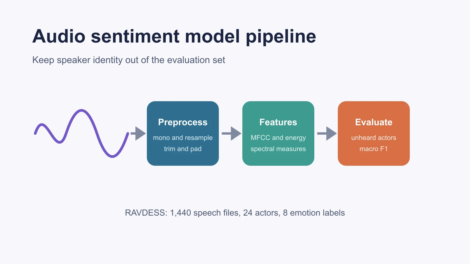 Machine Learning
Building a Sentiment Analysis Model With Audio Data
Build and evaluate an audio sentiment model in Python using RAVDESS, librosa features, actor-grouped validation, and honest emotion labels.
Sep 23, 2026
-
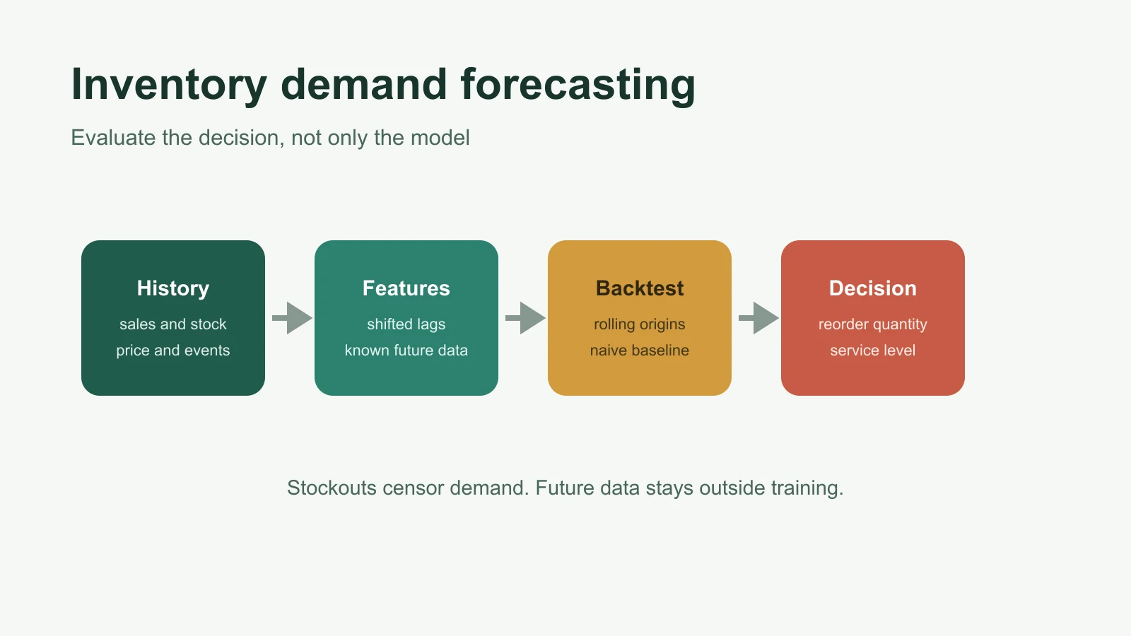 Machine Learning
Building an AI-Based Inventory Demand Forecasting Model
Build an inventory demand forecast in Python with leakage-safe lag features, rolling validation, seasonal baselines, practical metrics, and monitoring.
Sep 23, 2026
-
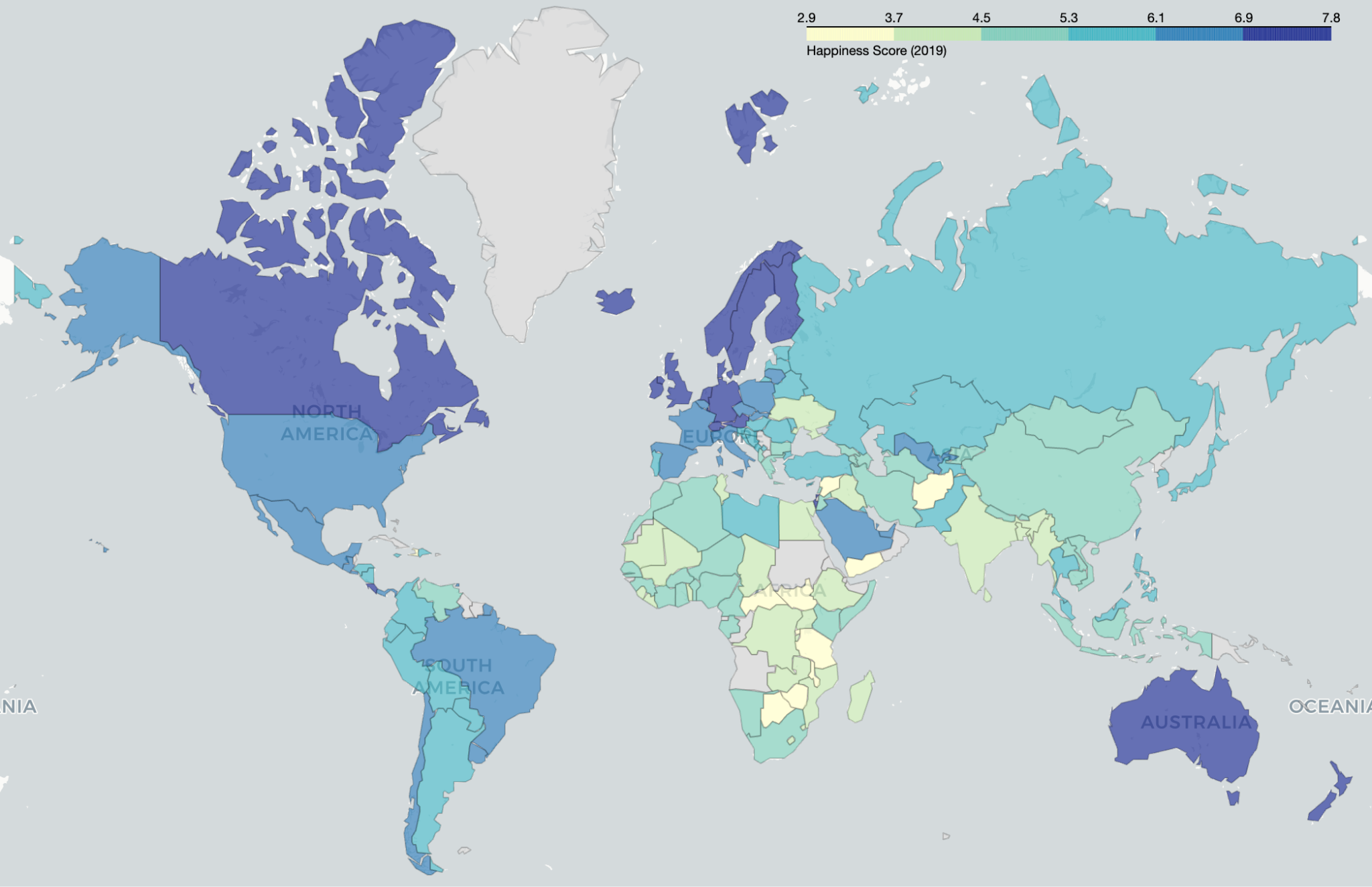 Python
World Happiness Report Analysis in Python: 9 Visualizations
Analyze the World Happiness Report 2019 in Python with pandas, seaborn, and Folium. 9 charts across 156 countries, and the two columns everyone misreads.
Aug 22, 2026