Case Study, Python
Python 2SLS Case Study: How Our Expert Helped a Student

An anonymized case study of a financial econometrics assignment completed with Python, macroeconomic data, and instrumental-variable estimation.
Written and technically reviewed by: Samuel P., Senior Python and ML Engineer Project type: Financial econometrics, Python, time-series data, and IV-2SLS Student privacy: This is a real project. The student’s name, university, grade, and deadline are withheld for privacy.
The assignment required more than a simple correlation
Samuel P., Senior Python and ML Engineer at GeeksProgramming, directly helped a financial econometrics student work through an assignment about the relationship between inflation and stock returns. The brief required a reduced-form derivation, a two-stage least squares analysis in Python, a written interpretation of the output, and short explanations of impulse response functions and forecast error variance decomposition.
The difficult part was the model structure. Inflation appeared in the stock returns equation, while stock returns appeared in the inflation equation. That feedback creates an endogeneity problem. A simple ordinary least squares regression could produce a neat table while still estimating the wrong relationship.
The project needed a report that connected the mathematics, data preparation, Python code, model output, and economic interpretation in one readable submission.
Project snapshot
| Project detail | Result |
|---|---|
| Assignment topic | The relationship between inflation and stock returns |
| Data period | April 1990 to March 2018 |
| Final analysis sample | 336 complete monthly observations |
| Main method | Instrumental-variable two-stage least squares |
| Python estimator | linearmodels.IV2SLS |
| Main deliverables | Reduced forms, Python code, two model summaries, interpretation, IRF and FEVD definitions |
The first step was to make the simultaneous model clear
The assignment used two structural equations. The first treated stock returns as an endogenous predictor of inflation. The second treated inflation as an endogenous predictor of stock returns:
inflation_t = α0 + α1 returns_t + α2 dcredit_t + α3 dprod_t + α4 dmoney_t + u1t

returns_t = β0 + β1 dprod_t + β2 dspread_t + β3 inflation_t + β4 rterm_t + u2t
The report then expressed both variables in reduced form using the exogenous variables from the system:
inflation = π10 + π11 dprod + π12 dcredit + π13 dmoney + π14 dspread + π15 rterm + v1

returns = π20 + π21 dprod + π22 dcredit + π23 dmoney + π24 dspread + π25 rterm + v2
The assignment instructions contained a typo in the textbook-style reduced-form specification. The solution removed qrev, as requested, and retained dprod, dcredit, dmoney, dspread, and rterm as the exogenous variables.
The Python workflow turned raw macro data into model variables
The supplied project included an Excel data file, a macro.pickle data file, a Python script, screenshots of the output, and the completed report. The code converted the monthly date field, created percentage changes, calculated the Treasury spread, and removed rows made incomplete by those transformations.
The final data set covered 336 monthly observations from April 1990 through March 2018. The code created these analysis variables:
returnsfrom percentage changes in the S&P 500 indexinflationfrom percentage changes in the Consumer Price Indexdprodfrom changes in industrial productiondmoneyfrom changes in M1 money supplydcreditfrom changes in consumer creditdspreadfrom the change in the Treasury yield spreadrtermfrom the three-month Treasury bill rate
The descriptive results gave the student a useful first look at the sample. Monthly inflation averaged 0.20 percent with a standard deviation of 0.33 percent. Monthly stock returns averaged 0.70 percent with a standard deviation of 4.09 percent. The simple correlation between inflation and returns was approximately -0.01, which already suggested that the simultaneous-equation models could tell a different story from a basic correlation table.
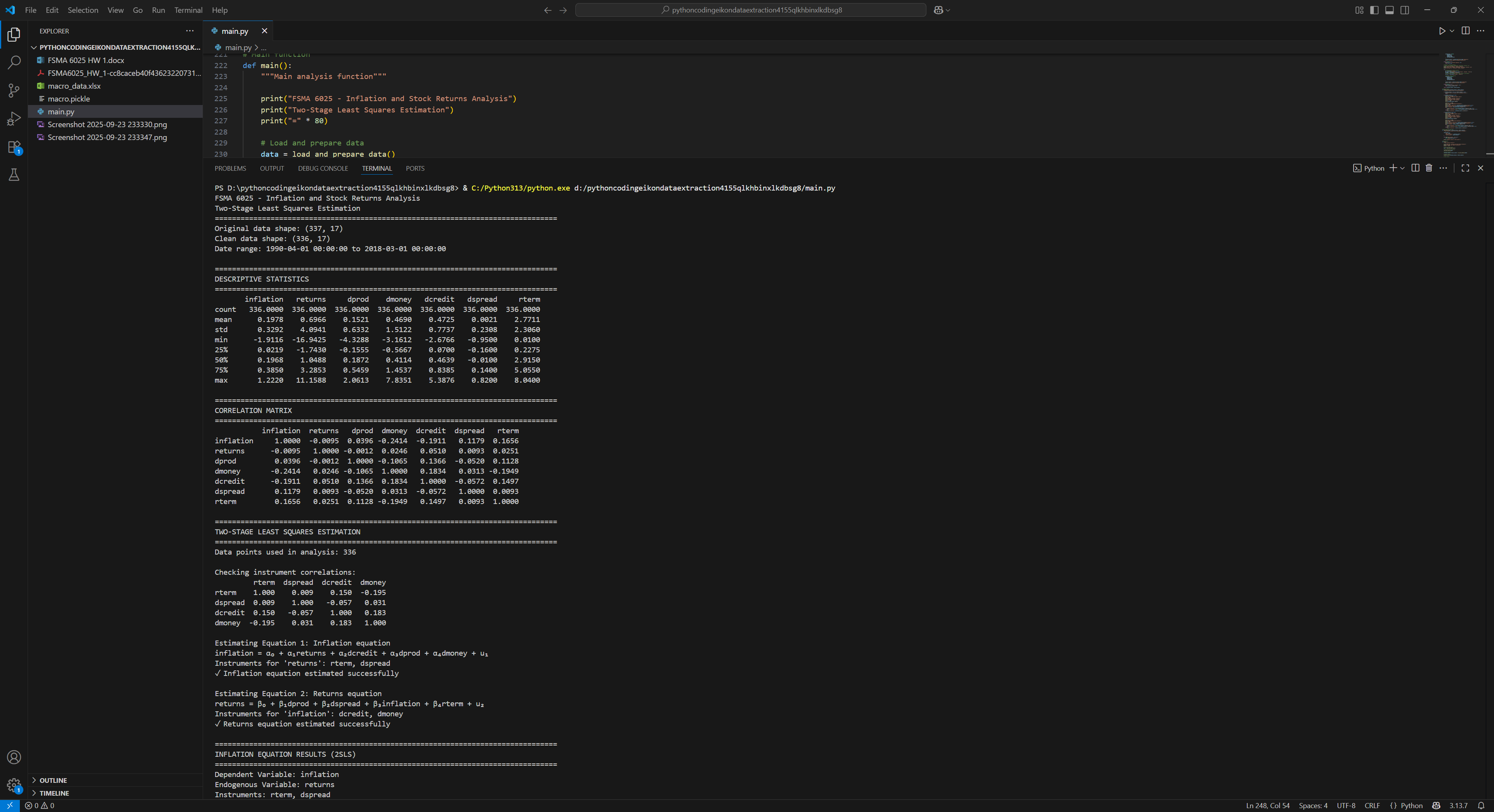
Figure 1. The supplied Python run shows 336 clean observations, the April 1990 to March 2018 date range, descriptive statistics, and the correlation matrix.
The instrument choices followed the equation being estimated
The analysis estimated each structural equation separately with an explicit endogenous variable and instrument list.
For the inflation equation, the code used returns as the endogenous variable. It used rterm and dspread as instruments, with dcredit, dprod, and dmoney as included exogenous variables.
For the returns equation, the code used inflation as the endogenous variable. It used dcredit and dmoney as instruments, with dprod, dspread, and rterm as included exogenous variables.
That setup made the identification strategy visible in the report instead of hiding it behind a single regression command. It also made the output easier to check against the equations in the assignment brief.
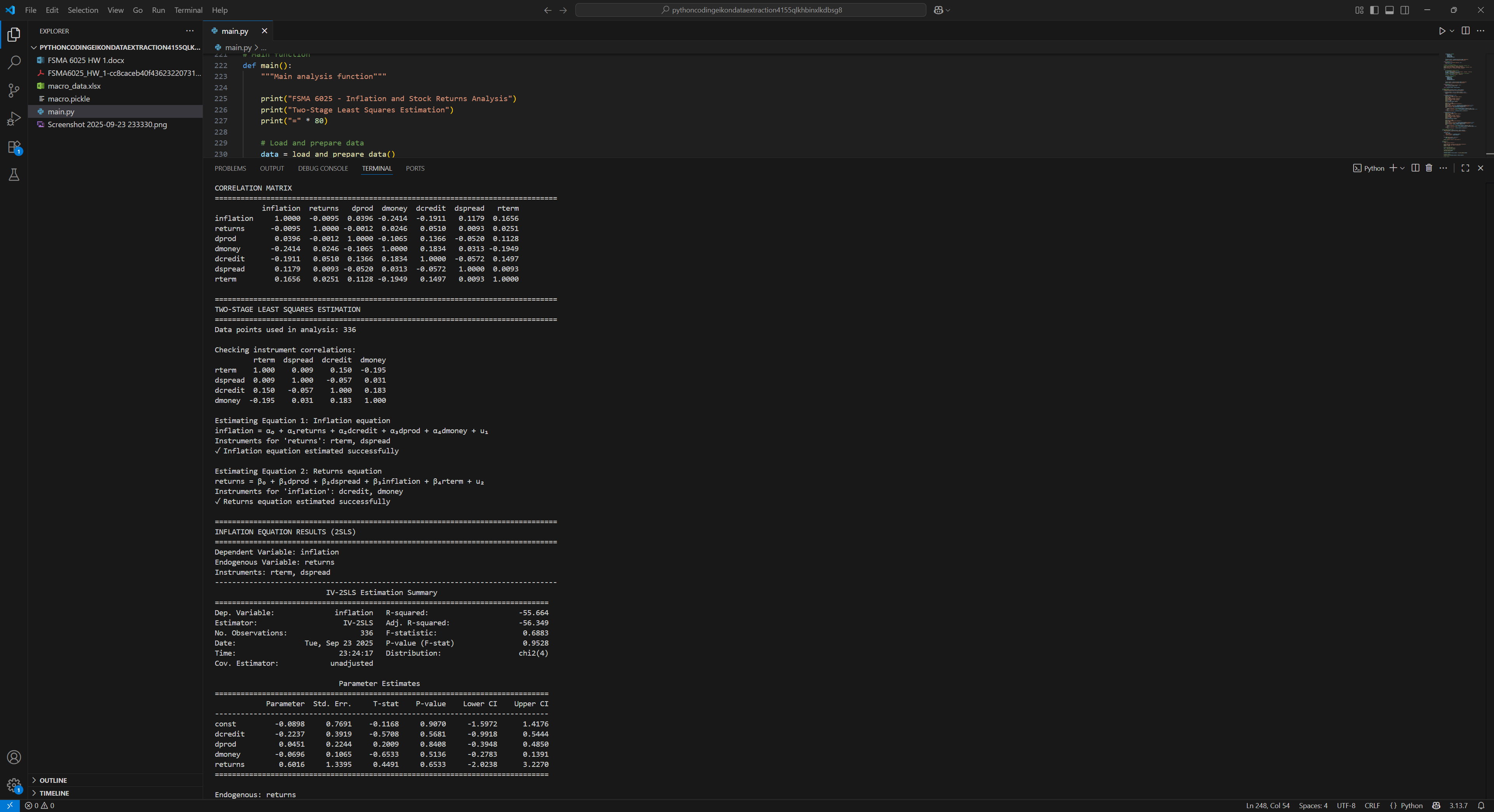
Figure 2. The execution screenshot shows the instrument-correlation check, both equation specifications, and the start of the inflation-equation results.
The 2SLS results did not support a statistically significant relationship
The fitted models produced different signs for the two endogenous coefficients, but neither coefficient was statistically significant.
| Structural relationship tested | Estimate | P-value | Interpretation at the 5% level |
|---|---|---|---|
| Stock returns to inflation | 0.6016 | 0.6533 | Not statistically significant |
| Inflation to stock returns | -2.2652 | 0.3643 | Not statistically significant |
In the inflation equation, the estimated coefficient on stock returns was positive, 0.6016, but its p-value was 0.6533. In the returns equation, the estimated coefficient on inflation was negative, -2.2652, with a p-value of 0.3643.
The correct conclusion was therefore limited and clear: the fitted sample did not provide statistically significant evidence of either endogenous relationship at the 5% or 10% level. The signs gave the student an economic story to discuss, but the p-values did not support a strong causal claim.
The IV summaries also reported R-squared values of -55.6644 for the inflation equation and -0.0258 for the returns equation. These are not ordinary OLS goodness-of-fit measures. They indicate that the chosen IV specifications fit the sample poorly under the reported metric and call for careful interpretation.
The report mentioned weak instruments and model specification as possible reasons for the weak results. It did not include first-stage F-statistics or over-identification tests, so this case study does not claim that instrument strength and validity were fully established. Those diagnostics would be sensible additions in a more advanced version of the analysis.
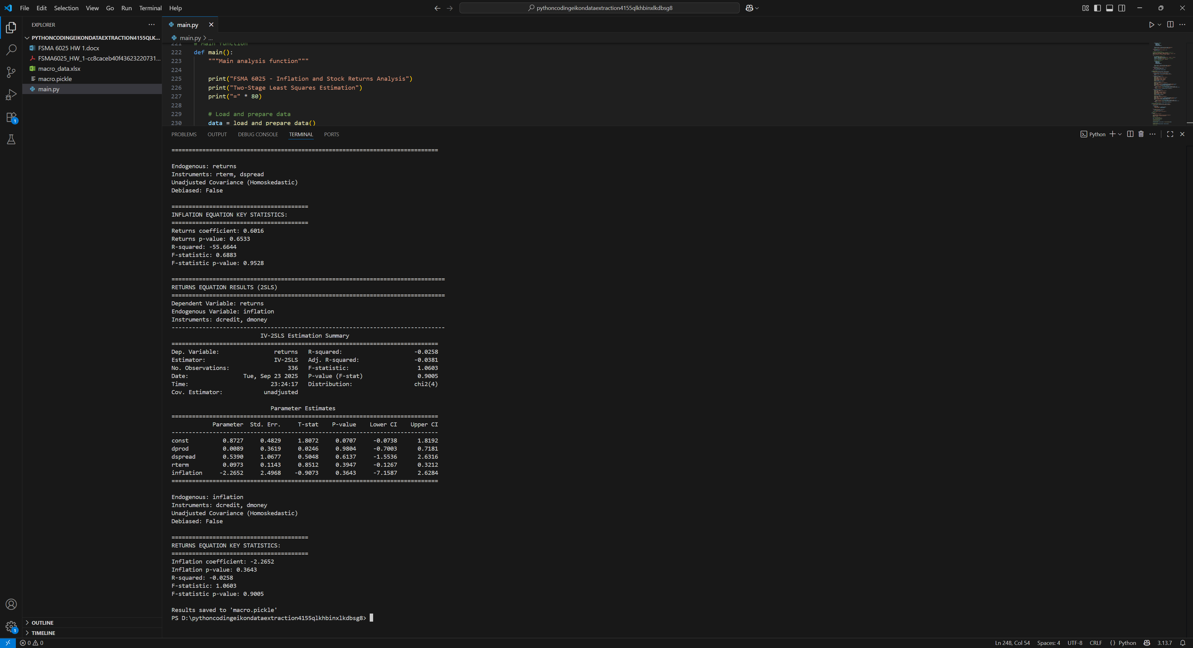
Figure 3. The final execution screenshot shows the key statistics for both equations and confirms that the analysis output was saved to macro.pickle.
The report explained two VAR concepts in plain language
The assignment also asked for definitions related to vector autoregression.
Impulse response function
An impulse response function shows how a variable responds over time after a shock to another variable in a VAR system. For example, an analyst can trace the effect of an unexpected inflation shock on stock returns across the following months. The response can be shown period by period or as a cumulative effect, depending on the specification.
Forecast error variance decomposition
Forecast error variance decomposition shows how much of a variable’s forecast uncertainty comes from shocks to each variable in the VAR. At a selected forecast horizon, the percentages add to 100 percent. An impulse response shows the path of a response; variance decomposition shows the relative contribution of each shock to forecast uncertainty.
What GeeksProgramming helped the student organize
The finished project brought several pieces together:
- a reduced-form explanation that matched the simultaneous-equation model;
- a reproducible Python data-preparation workflow;
- explicit IV-2SLS specifications for both structural equations;
- result tables with coefficient estimates, standard errors, test statistics, and p-values;
- an interpretation that did not confuse a coefficient sign with statistical evidence;
- concise explanations of impulse responses and forecast error variance decomposition.
The completed project package contains the three-page report, the Python source file, the input data, the saved pickle file, and screenshots of the execution output. That gives the work a traceable path from data preparation to final interpretation.
The main lesson was careful interpretation
This assignment showed why econometrics reports need more than code that runs. The model had a feedback relationship, so the student had to identify endogenous variables and choose instruments. The data had to be transformed before estimation. The output then required a conclusion that respected the p-values rather than overstating the result.
The final analysis did not find statistically significant evidence that inflation and stock returns affected one another in the specified sample and model. That is a valid result. A careful report explains it, shows how it was obtained, and identifies the diagnostics that could strengthen a follow-up study.
Students working on a similar Python or econometrics assignment can contact GeeksProgramming for help with data preparation, model implementation, output interpretation, and report structure. Support should leave the student able to explain the method and defend the result in their own words.
Frequently asked questions
What was the assignment about?
It examined the relationship between inflation and stock returns with a simultaneous-equation model, IV-2SLS estimation, and two short VAR concept questions.
How much data did the analysis use?
The cleaned sample contained 336 monthly observations from April 1990 through March 2018.
Which Python package estimated the models?
The project used linearmodels.IV2SLS with unadjusted covariance estimates.
Were the inflation and stock returns coefficients statistically significant?
No. The reported p-values were 0.6533 for stock returns in the inflation equation and 0.3643 for inflation in the stock returns equation.
Privacy and evidence note
This is a real GeeksProgramming project handled with Samuel P. The case study is based on the assignment brief, report, Python script, data files, and three execution screenshots. The student’s name, university, grade, deadline, and private submission details are withheld for privacy.