Case Study, Machine Learning
Python Neural Networks for Surface Hardness and Roughness

A worked Mechanics of Advanced Manufacturing case study
Project type: Python machine-learning assignment Methods: Exploratory data analysis, StandardScaler, TensorFlow/Keras, Adam, early stopping, grid search Outputs: Surface hardness in HV and final surface roughness, Ra Data basis: 5,000 synthetic samples generated from published empirical equations
This case study follows a student project that used Python to predict two outcomes from a turn-assisted deep cold rolling process: surface hardness and final roughness. The interesting part was not simply fitting a neural network. The assignment required two modeling strategies, a defensible hyperparameter search, evidence of convergence, and a clear explanation of what the results mean.
The supplied solution met that structure. It generated 5,000 samples from the equations in Section 3.5 of the assigned research paper, trained three model families, compared 54 network configurations per family, and evaluated the selected models on a 20% holdout set. The results are strong because the networks learned a deterministic mathematical relationship. They are not a replacement for new machining experiments.
The assignment asked for two prediction strategies
The assignment focused on the turn-assisted deep cold rolling of AISI 4140 steel. Each row of the modeling data used four process inputs:
- X1: rolling ball diameter in millimeters
- X2: rolling force in newtons
- X3: initial surface roughness, Ra, in micrometers
- X4: number of rolling passes
The prediction targets were surface hardness, HV, and final surface roughness, Ra. The student had to compare two approaches:
- Train one neural network for hardness and a second neural network for roughness.
- Train one multi-output neural network that predicts both targets at the same time.
The assignment also specified the decisions that needed testing: hidden-layer count, neurons per layer, activation function, and dropout ratio. Adam was the optimizer, and early stopping was required for every model.
That combination makes this a useful Python assignment case study. It tests data preparation, model design, experiment tracking, and interpretation in one workflow.
The expert started with a transparent synthetic dataset
The notebook implemented the supplied surface-hardness and surface-finish equations as two Python functions, hv() and ra(). It then sampled process inputs over the selected operating ranges and calculated the two target columns from those equations. There was no hidden dataset and no claim that the 5,000 rows came from a new laboratory experiment.
The workflow produced an 80/20 development and test split: 4,000 rows for model development and 1,000 rows for final holdout evaluation. A fixed random seed of 7 made the run repeatable. For the EDA section, the notebook inspected a reproducible random sample of 500 rows rather than plotting every generated row at once.
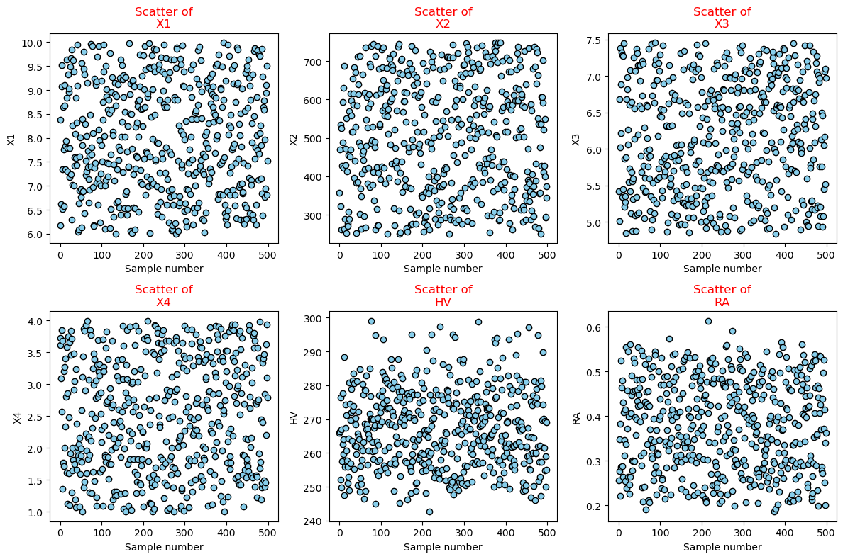
Figure 1. The notebook’s 500-row EDA sample. The first four panels show the input factors; the bottom panels show generated hardness and roughness values.
The source paper contains real machining experiments and response-surface modeling. This student project used the paper’s equations as instructed, which gives the neural network a controlled way to learn the stated response surface. That distinction matters when the final results are explained to a student or instructor.
EDA showed which inputs mattered most
The exploratory charts made the data easier to reason about before training. The distributions cover the intended input ranges without an obvious empty band, and the target values stay in plausible ranges for the supplied equations.
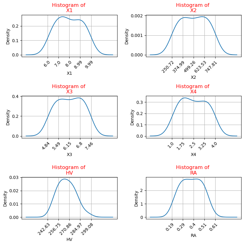
Figure 2. Distribution checks for the generated modeling data. The plots help confirm that the sampled inputs and equation outputs are present across the working range.
The correlation matrix provided a useful first read of the response surface:
- Rolling force, X2, had the strongest positive linear association with hardness in the sample, at approximately 0.83.
- Number of passes, X4, had a strong negative linear association with final roughness, at approximately -0.97.
- Hardness and roughness had a negative association of approximately -0.35.
These numbers describe the generated sample. They are not causal estimates from a fresh experiment. They still helped the expert check whether the neural-network outputs followed the broad patterns implied by the empirical equations.
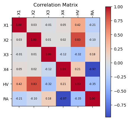
Figure 3. Correlations in the 500-row EDA sample. The heatmap is a diagnostic view, not a substitute for the model and the source equations.
The input-output plots added a second layer of interpretation. Hardness generally increased with ball diameter and rolling force, while roughness fell as the number of passes increased. The curves are not straight lines in every panel because the equations contain interaction terms and nonlinear combinations of the inputs.
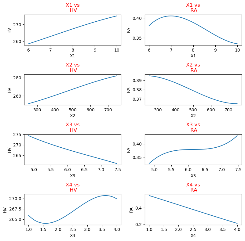
Figure 4. The generated response patterns across each input factor. The plots reflect one-variable-at-a-time visualizations, so interactions still need to be considered in the full model.
Standardization kept the inputs on a common scale
The notebook used StandardScaler from scikit-learn. It fitted the scaler on the training inputs only, then applied the same transformation to the test inputs. That order is important because fitting the scaler on all rows would allow test-set information to influence the training pipeline.
The four inputs have very different numerical scales. Rolling force is measured in hundreds of newtons, while ball diameter is measured in single-digit millimeters. Standardization places them on a comparable scale before the dense layers process them. The targets were kept in their original units so the final MSE values remained interpretable as hardness and roughness errors.
A 54-model grid made the architecture choice explicit
Each model family used the same search space:
| Hyperparameter | Values tested |
|---|---|
| Hidden layers | 1, 2, 3 |
| Neurons per hidden layer | 16, 32, 64 |
| Activation | ReLU, tanh, sigmoid |
| Dropout ratio | 0.0, 0.2 |
| Optimizer | Adam |
| Maximum epochs | 1,000 |
| Early-stopping patience | 50 epochs |
The grid contained 54 combinations for each model family. The notebook therefore trained 162 candidate networks across the two single-output models and the multi-output model. Each candidate used mean squared error as its loss and reported MSE and R².
One practical result stood out: the zero-dropout models dominated the best part of the grids. For this deterministic, equation-generated dataset, dropping 20% of hidden activations made the fit less precise rather than improving generalization. That is a useful lesson for students: regularization is a tool to test, not an automatic improvement.
The separate models and the multi-output model both converged
The selected configurations were:
| Model | Prediction target | Hidden layers | Neurons | Activation | Dropout |
|---|---|---|---|---|---|
| Model 1 | Surface hardness, HV | 3 | 16 | sigmoid | 0.0 |
| Model 2 | Final roughness, Ra | 1 | 16 | tanh | 0.0 |
| Model 3 | HV and Ra together | 2 | 64 | sigmoid | 0.0 |
The separate hardness model recorded a training MSE of 0.001789 and a test MSE of 0.002157, with R² values of 0.999985 and 0.999984. The separate roughness model recorded a training MSE of approximately 6.45 × 10⁻⁷ and a test MSE of approximately 6.67 × 10⁻⁷, with R² values of 0.999932 on both sets.
The multi-output model produced a training MSE of 0.000495 and a test MSE of 0.000504. Its average R² was 0.999524 on the training data and 0.999486 on the test data. The combined MSE is influenced by the different scales of HV and Ra, so the per-target R² values and the separate model results provide the clearer comparison.
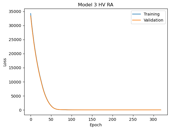
Figure 5. Training and validation loss for Model 3. The curves fall together and level off without a visible validation rise, which supports the report’s finding that the selected model did not show meaningful overfitting on this holdout split.
The small gap between training and test metrics is consistent with the data-generation setup. Both sets were sampled from the same equations and operating ranges. It supports convergence for this modeling exercise, but it does not establish how the model behaves on noisy measurements, a different material, or a process outside the sampled range.
The test predictions followed the equation-generated targets
The selected networks produced near-diagonal actual-versus-predicted plots on the holdout data. That visual pattern agrees with the reported R² values. It also gives students a more intuitive way to read the metrics: points close to the diagonal indicate that the prediction tracks the target value across the test range.
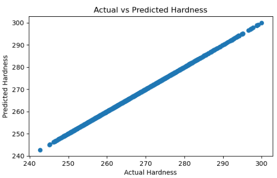
Figure 6. Model 1 hardness predictions on 1,000 holdout rows. The diagonal pattern shows close agreement with the equation-generated target values.
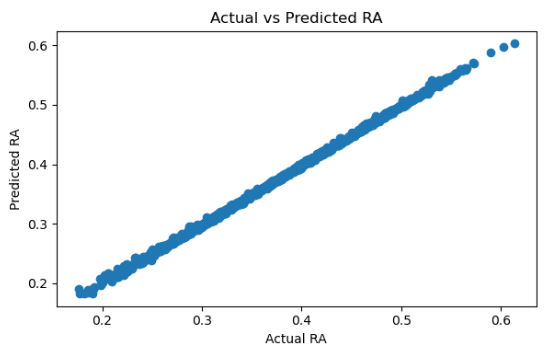
Figure 7. Model 2 roughness predictions on the holdout set. The axes use final roughness, Ra, for both the target and prediction.
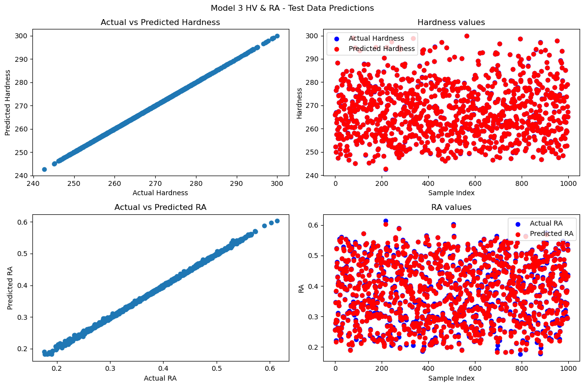
Figure 8. Model 3 predictions for both responses. The left column compares actual and predicted values; the right column shows the two series across the holdout sample index.
What the results mean for a student
The strongest part of this solution is the chain of evidence. The notebook does not stop at a single impressive R² value. It shows how the data was generated, checks the distributions, scales the inputs, tests the requested architecture choices, selects a configuration, plots training and validation loss, and evaluates the selected network on rows it did not train on.
That sequence gives a student a repeatable pattern for other Python machine-learning assignments:
- Translate the assignment into clearly named inputs, outputs, and units.
- Make the data source explicit before training a model.
- Use a fixed split and a fixed random seed so the run can be checked.
- Compare hyperparameters with a table instead of choosing a network by guesswork.
- Show both numerical metrics and visual predictions.
- Explain what the metric proves and what it does not prove.
For students looking for programming assignment help, this is the difference between a notebook that runs and a project that can be explained in a report or viva. Students working on neural networks, regression, or engineering data can also explore focused Python assignment help for support with similar coursework.
Important note about the dataset and results
The case study describes the supplied notebook as it ran. One range deserves a final instructor check: the notebook samples the number of passes, X4, uniformly from 1 to 4, while the reference paper’s Table 2 lists 1, 2, and 3 as the three experimental levels. The other three input ranges match the low-to-high values shown in that table. If the instructor expects the exact reference levels, the student should confirm whether X4 was intended to be sampled from 1 to 3 before submitting the notebook.
That note does not change the interpretation of the figures above. It simply keeps the case study honest about the difference between the reference design and the supplied implementation.
The results also need to be described with the right scope. The 5,000 rows are synthetic, equation-generated training examples. The neural networks learned the supplied empirical response surface with very small holdout error. They did not produce new measurements of a rolled AISI 4140 steel shaft, and the case study does not present them as experimental proof.
Source and learning context
The equations came from P. R. Prabhu, S. M. Kulkarni, and S. Sharma, “Multi-response optimization of the turn-assisted deep cold rolling process parameters for enhanced surface characteristics and residual stress of AISI 4140 steel shafts,” Journal of Materials Research and Technology, 9(5), 11402-11423, 2020. The assigned source is available through the paper DOI.
This page is an anonymized learning case study. It does not publish the student’s name or university, and it uses the project outputs supplied for the case. Students can use the structure to understand their own work, then cite the original paper and write their own explanation of the code and results.