Building an AI-Based Inventory Demand Forecasting Model

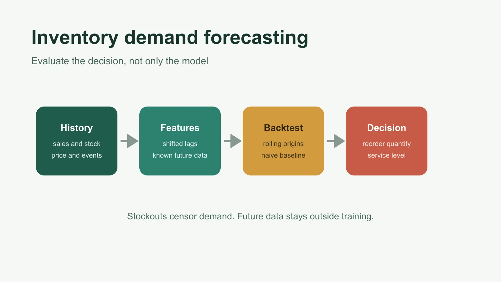
Forecasting inventory demand helps a business cut stockouts without piling up excess stock. Machine learning can combine sales history with price, promotions, seasonality, and product information, but the algorithm is only one part of the project. This guide moves from problem definition and data collection to feature engineering, model evaluation, deployment, and monitoring.

Define the inventory decision and forecast grain

Begin by specifying the item, location, time bucket, horizon, and decision that consumes the prediction. “Forecast demand” is incomplete until those five attributes are fixed.

Consider a retailer that orders every Monday, receives stock after 14 days, and sells through 12 stores. Its useful target is not total monthly sales. It needs daily demand for each SKU-store pair across at least the next 14 days, followed by an aggregation that matches the ordering rule.

Design choice	Example	Why it matters
Item	SKU	Different products have different life cycles
Location	Store	Local demand and stock constraints differ
Time bucket	Day	Promotions and weekday effects stay visible
Horizon	14 days	Covers supplier lead time
Decision	Reorder quantity	Converts a forecast into inventory action

A horizon is part of the target. A model evaluated one day ahead does not establish 14-day replenishment performance.

Separate observed sales from true demand

Sales history forms the foundation of the model, but it does not always equal demand. First identify the periods when inventory availability limited sales. When stock reaches zero, observed sales become a censored lower bound on what customers wanted.

Suppose a product usually sells 12 units on Saturdays. It sells 3 units before running out at noon. Training on 3 tells the model that Saturday demand fell, exactly when demand may have exceeded supply. Promotions, store closures, listing changes, returns, and substitutions create similar gaps between recorded transactions and the forecasting target.

Create explicit fields such as in_stock, stockout_hours, promotion, price, store_open, and product_active. A classroom model can exclude fully stocked-out targets and disclose that choice. A production system needs lost-sales estimation, availability-aware likelihoods, or another method that models censoring directly.

Build a clean SKU-location time series

Create one row for every expected date, SKU, and location, including zero-sales days. A missing row and a recorded zero are different facts.

The working table uses this schema:

date,sku,store,units,price,promotion,stock_on_hand
2026-01-01,SKU-104,STORE-03,12,8.99,0,46
2026-01-02,SKU-104,STORE-03,15,8.99,0,31
2026-01-03,SKU-104,STORE-03,0,8.99,0,0

Validate the following before feature engineering:

uniqueness of date + sku + store;
nonnegative unit counts and inventory balances;
consistent time zones and business-day boundaries;
product launch and discontinuation dates;
promotion start and end dates;
gaps caused by missing feeds or closed stores;
returns stored separately from gross demand.

Do not replace every missing unit value with zero. Zero means observed no demand; missing means unknown.

Explore demand at 4 useful levels

Exploratory analysis works best at four levels: total, item, location, and item-location. Aggregated demand can look smooth while individual SKUs remain sparse or volatile.

Plot total units by day to find trend, holidays, and system outages.
Plot units by SKU to find launches, decline, and intermittent demand.
Compare stores to find local calendars and assortment differences.
Calculate the proportion of zero days for every SKU-store series.

Add price and promotion overlays. A spike during a discount is not unexplained seasonality. Mark stockouts on the same plot because a sudden zero with no inventory has a different cause from a zero with stock available.

Establish seasonal-naive and moving-average baselines

A forecasting model earns its complexity by beating a rule that a planner could use without machine learning. For daily retail demand, a seasonal-naive baseline predicts the value observed 7 days earlier.

import pandas as pd

sales = pd.read_csv("data/daily_sales.csv", parse_dates=["date"])
keys = ["sku", "store"]
sales = sales.sort_values(keys + ["date"])

sales["naive_7"] = sales.groupby(keys)["units"].shift(7)
sales["moving_28"] = sales.groupby(keys)["units"].transform(
    lambda series: series.shift(1).rolling(28, min_periods=7).mean()
)

The shift is essential. A rolling mean without shift(1) includes the current target in its own feature. That leak produces impressive validation scores and impossible production inputs.

The forecast-accuracy guidance in Forecasting: Principles and Practice recommends evaluating genuine forecasts on data that did not fit the model. A candidate that cannot beat the seasonal-naive rule does not justify extra deployment cost.

Engineer lag, rolling, calendar, and commercial features

Feature engineering turns sales history and business context into model inputs. Build each feature from information available at the forecast timestamp; every column needs an availability test, not merely a correlation with demand.

import numpy as np

grouped = sales.groupby(keys, group_keys=False)

for lag in (1, 7, 14, 28):
    sales[f"lag_{lag}"] = grouped["units"].shift(lag)

for window in (7, 28):
    sales[f"mean_{window}"] = grouped["units"].transform(
        lambda series: series.shift(1).rolling(window, min_periods=4).mean()
    )
    sales[f"std_{window}"] = grouped["units"].transform(
        lambda series: series.shift(1).rolling(window, min_periods=4).std()
    )

sales["day_of_week"] = sales["date"].dt.dayofweek
sales["month"] = sales["date"].dt.month
sales["week_of_year"] = sales["date"].dt.isocalendar().week.astype(int)
sales["price_change"] = grouped["price"].pct_change().replace([np.inf, -np.inf], np.nan)

Known-future features can include an approved promotion calendar, planned price, store closures, and holidays. Unknown-future features cannot be filled from realized values during backtesting. Weather forecasts available at prediction time differ from final observed weather.

Keep one feature-availability table

Document when each feature becomes available. This small table prevents some of the hardest leakage bugs to notice.

Feature	Available for future dates?	Safe use
Day of week	Yes	Every horizon
Approved promotion	Yes	Dates covered by the promotion plan
Actual future price	No	Replace with planned price
Lagged units	Only through forecast origin	Use observed history, then recursive predictions for longer horizons
Final weather observation	No	Use the archived forecast issued at the origin
Stock received tomorrow	Only if scheduled	Use confirmed purchase-order data

Split the data by time, never at random

Training data comes from earlier dates and evaluation data comes from later dates. A random split lets tomorrow teach yesterday and mixes seasonal regimes across both sets.

Use rolling-origin validation: choose several forecast origins, train only on rows before each origin, and score the next horizon. The time-series cross-validation description formalizes this rule by ensuring that every test observation occurs after its training observations.

from pandas.tseries.offsets import Day


def rolling_origins(data, origins, horizon_days=14):
    for origin in origins:
        train = data[data["date"] < origin]
        valid = data[
            (data["date"] >= origin)
            & (data["date"] < origin + Day(horizon_days))
        ]
        yield origin, train, valid

Choose origins that cover ordinary weeks, promotions, and seasonal peaks. Keep the newest block as a final untouched test period after model selection.

Train a global count model in Python

A global model shares information across related series by combining SKU and store identifiers with lagged features. A Poisson-loss gradient booster respects nonnegative count targets better than ordinary squared-error regression in many retail settings.

from sklearn.compose import ColumnTransformer
from sklearn.ensemble import HistGradientBoostingRegressor
from sklearn.pipeline import make_pipeline
from sklearn.preprocessing import OneHotEncoder

categorical = ["sku", "store"]
numeric = [
    "price",
    "promotion",
    "day_of_week",
    "month",
    "week_of_year",
    "lag_1",
    "lag_7",
    "lag_14",
    "lag_28",
    "mean_7",
    "mean_28",
    "std_7",
    "std_28",
]

preprocess = ColumnTransformer(
    [("category", OneHotEncoder(handle_unknown="ignore", sparse_output=False), categorical)],
    remainder="passthrough",
)

model = make_pipeline(
    preprocess,
    HistGradientBoostingRegressor(
        loss="poisson",
        learning_rate=0.05,
        max_iter=300,
        max_leaf_nodes=31,
        l2_regularization=1.0,
        random_state=42,
    ),
)

train_rows = train.dropna(subset=numeric + ["units"])
model.fit(train_rows[categorical + numeric], train_rows["units"])

This model is a baseline, not a universal winner. Intermittent demand may favor Croston-family methods. Smooth seasonal series may favor exponential smoothing. Large assortments with rich covariates may benefit from boosted trees or neural forecasting. Backtesting at the required horizon decides.

Do not use realized lags in a multi-day forecast

A 14-day forecast from one origin requires recursive lag updates or a direct model for each horizon. Using the actual units from day 1 to predict day 2 is valid only after day 1 has occurred. It is leakage when all 14 predictions were supposedly issued together.

Three strategies fit different needs:

Recursive: predict one step, append it, rebuild lags, and repeat. Errors can accumulate.
Direct: train a separate target for each horizon. Compute and maintenance increase.
Multi-output: predict the full horizon together. Cross-horizon structure is explicit but model design is more complex.

Record the issue timestamp for every forecast. Evaluation then reconstructs exactly what information existed at that moment.

Evaluate error, bias, and inventory consequences

Compare models with MAE, WAPE, bias, and horizon-specific error against the same baseline. MAPE is unstable when actual demand is zero and can over-weight small-volume items.

import numpy as np
from sklearn.metrics import mean_absolute_error


def forecast_metrics(actual, predicted):
    actual = np.asarray(actual)
    predicted = np.clip(np.asarray(predicted), 0, None)
    error = predicted - actual

    return {
        "mae": mean_absolute_error(actual, predicted),
        "wape": np.abs(error).sum() / max(actual.sum(), 1),
        "bias": error.sum() / max(actual.sum(), 1),
    }

MAE stays in unit terms. WAPE summarizes total absolute error relative to total demand. Bias shows systematic over- or under-forecasting. Calculate each by horizon, SKU volume band, store, category, promotion status, and stock-availability status.

A statistically smaller error may not reduce cost. Translate forecasts into the replenishment policy and simulate stockouts, waste, holding cost, and service level. Under-forecasting a critical part and over-forecasting a low-cost staple do not carry the same consequence.

Add uncertainty to the replenishment decision

Safety-stock planning needs prediction intervals or quantile forecasts rather than one point. A 90th-percentile forecast is useful when the cost of a stockout exceeds the cost of carrying extra inventory.

Check interval coverage by horizon and product group. An interval that claims 90 percent coverage but contains only 65 percent of future observations understates risk. Also check width: an interval can achieve coverage by becoming too broad to guide a decision.

Use the service-level target and lead-time variability to choose the operational quantile. The forecast model and inventory policy are separate components, so evaluate them together.

Monitor the data, forecast, and decision layers

Once the model is deployed, monitor input freshness, feature distributions, error, bias, interval coverage, and inventory outcomes. One dashboard cannot replace those distinct checks.

Data layer: missing feeds, duplicate rows, price anomalies, delayed promotions.
Forecast layer: MAE, WAPE, bias, interval coverage, baseline skill.
Decision layer: fill rate, stockout hours, excess inventory, waste, holding cost.

Retrain on a schedule justified by demand change and data arrival. Trigger investigation when bias persists across several forecast origins or when the candidate loses to the seasonal-naive model.

Use a reproducible project structure

A reviewable project preserves raw data, split definitions, features, forecasts, and evaluation outputs separately.

inventory-forecast/
├── data/
│   ├── raw/
│   ├── processed/
│   └── forecast-origins.csv
├── src/
│   ├── validate.py
│   ├── features.py
│   ├── train.py
│   ├── forecast.py
│   └── evaluate.py
├── reports/
│   ├── baseline-comparison.csv
│   ├── error-by-horizon.csv
│   └── inventory-simulation.csv
├── models/
├── requirements.txt
└── README.md

Students can use machine learning assignment help to review the backtest, Python assignment help to debug the feature pipeline, or statistics homework help to interpret uncertainty and forecast error. The finished report needs to explain why each split, metric, and feature matches the replenishment decision.

Questions about inventory demand forecasting

What data is required for inventory forecasting?

The minimum dataset contains timestamped units by SKU and location. Stronger systems add inventory availability, price, promotions, product status, holidays, store closures, supplier lead times, and confirmed future events.

Why is a random train-test split wrong for demand data?

A random split mixes future and past observations. It gives the model information from later seasonal regimes and produces an evaluation that does not match real forecasting.

Which baseline fits daily retail demand?

A 7-day seasonal-naive forecast is a useful first baseline when weekday patterns exist. Also compare a recent moving average and a zero or last-value rule for intermittent items.

Why can sales underestimate demand?

Sales stop when inventory is unavailable, even when customers still want the product. Stockout periods therefore censor demand and can teach a model that popular items have low demand.

Is MAPE suitable when demand contains zeros?

No. Percentage error is undefined at zero and unstable near zero. MAE, WAPE, MASE, or RMSSE provide more useful comparisons, depending on the portfolio and decision.

Which algorithm is best for inventory forecasting?

No algorithm wins across every assortment. Compare seasonal-naive, moving-average, statistical, tree-based, and specialized intermittent-demand methods using rolling-origin validation at the required horizon.

How often does a demand model require retraining?

Retraining frequency depends on data volume, seasonality, assortment changes, and drift. Track rolling error and bias, then retrain when new data materially improves a validated candidate.

How does a forecast become a reorder quantity?

The inventory policy combines demand across lead time with current stock, open purchase orders, safety stock, order constraints, and service-level targets. The point forecast alone is not the order.