Building a Sentiment Analysis Model With Audio Data

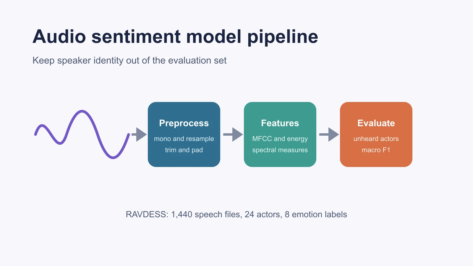
Sentiment analysis is widely used to understand customer feedback and conversations, yet most introductory projects focus only on text. Voice adds tone, pitch, energy, and timing, which can reveal information that a transcript misses. This guide walks through the full project, from dataset to evaluation, and settles one label issue first: RAVDESS contains acted emotions, so the first model performs speech-emotion recognition before we discuss genuine positive, neutral, and negative sentiment.

Define the prediction target before touching the audio

The project begins by deciding whether the target is emotion, sentiment, or both. These labels answer different questions.

• Emotion recognition predicts states such as happy, sad, angry, fearful, calm, or surprised from vocal expression.
• Sentiment analysis predicts an attitude such as positive, neutral, or negative toward an entity or topic.
• Multimodal sentiment analysis combines acoustic features with spoken words and sometimes video.

A cheerful tone does not guarantee positive sentiment. A speaker can happily describe a competitor’s failure, and a tired speaker can praise a product. Acoustic features reveal delivery; a transcript reveals semantic content. Treating one as the other creates label noise before training begins.

For RAVDESS, keep the eight supplied speech-emotion classes as the primary target. Collapse them into 3 sentiment classes only when the project specification defines the mapping and acknowledges ambiguous states such as surprise and calm.

Use RAVDESS as a controlled learning dataset

For a reproducible starting point, use the audio-only speech portion of the RAVDESS dataset. Its documented speech archive contains 1,440 WAV files from 24 professional actors, with 60 trials per actor. The actors speak two lexically matched statements in a neutral North American accent and perform eight emotions at normal or strong intensity where applicable.

RAVDESS is valuable for learning because its filenames encode the labels and speaker identity. It is limited because the performances are acted, the language and accent range is narrow, and the same two statements repeat throughout the speech subset. A high score on this dataset does not establish performance on spontaneous calls, clinical speech, podcasts, or multilingual conversations.

The dataset uses a Creative Commons Attribution-NonCommercial-ShareAlike 4.0 license and offers separate commercial licensing. Check the license before deploying a trained model outside coursework or research.

Decode the seven fields in each filename

RAVDESS places seven fields in every filename. Split the stem on hyphens to read them. A name such as 03-01-05-02-02-01-12.wav encodes audio-only modality, speech, angry emotion, strong intensity, statement 2, repetition 1, and actor 12.

from dataclasses import dataclass
from pathlib import Path

EMOTIONS = {
    "01": "neutral",
    "02": "calm",
    "03": "happy",
    "04": "sad",
    "05": "angry",
    "06": "fearful",
    "07": "disgust",
    "08": "surprised",
}


@dataclass(frozen=True)
class RavdessLabel:
    path: Path
    emotion: str
    actor: int
    intensity: int


def parse_ravdess(path: Path) -> RavdessLabel:
    fields = path.stem.split("-")
    if len(fields) != 7:
        raise ValueError(f"Unexpected RAVDESS filename: {path.name}")

    modality, channel, emotion, intensity, _, _, actor = fields
    if modality != "03" or channel != "01":
        raise ValueError("This project expects audio-only speech files")

    return RavdessLabel(
        path=path,
        emotion=EMOTIONS[emotion],
        actor=int(actor),
        intensity=int(intensity),
    )

The parser rejects video and song files instead of silently mixing modalities. That validation prevents a folder mistake from changing the task.

Split by actor to stop identity leakage

Keep all recordings from one actor inside one split when measuring performance on unheard speakers. A random file-level split places the same voice, microphone conditions, and speaking habits in both training and test data. The classifier can exploit speaker identity instead of learning emotion patterns that transfer.

This is a grouped-data problem. The independent unit is the actor, not the WAV file.

from pathlib import Path
from sklearn.model_selection import GroupShuffleSplit

records = [parse_ravdess(path) for path in Path("data/ravdess").rglob("*.wav")]

paths = [record.path for record in records]
labels = [record.emotion for record in records]
groups = [record.actor for record in records]

outer_split = GroupShuffleSplit(n_splits=1, test_size=0.20, random_state=42)
train_valid_idx, test_idx = next(outer_split.split(paths, labels, groups))

train_valid_paths = [paths[i] for i in train_valid_idx]
train_valid_labels = [labels[i] for i in train_valid_idx]
train_valid_groups = [groups[i] for i in train_valid_idx]

inner_split = GroupShuffleSplit(n_splits=1, test_size=0.25, random_state=42)
train_idx, valid_idx = next(
    inner_split.split(train_valid_paths, train_valid_labels, train_valid_groups)
)

train_paths = [train_valid_paths[i] for i in train_idx]
train_labels = [train_valid_labels[i] for i in train_idx]
valid_paths = [train_valid_paths[i] for i in valid_idx]
valid_labels = [train_valid_labels[i] for i in valid_idx]

With 24 actors, a 20 percent test split contains about 5 held-out speakers. Class proportions can vary because groups are indivisible. Record the actor IDs and class counts in every split, then keep the test set sealed until model selection is complete.

The scikit-learn leakage guidance explains the general rule: data used to evaluate a model cannot influence fitting or preprocessing. Actor grouping applies that rule to repeated speech samples.

Standardize audio without erasing the target

Audio preparation converts each file to mono, resamples it consistently, trims excessive silence, and normalizes only when the operation matches deployment conditions. Apply the same function to training, validation, test, and future inputs.

import librosa
import numpy as np


def load_audio(path, sample_rate=16_000, duration=3.0):
    signal, _ = librosa.load(path, sr=sample_rate, mono=True)
    signal, _ = librosa.effects.trim(signal, top_db=30)

    target_length = int(sample_rate * duration)
    if len(signal) < target_length:
        signal = np.pad(signal, (0, target_length - len(signal)))
    else:
        signal = signal[:target_length]

    peak = np.max(np.abs(signal))
    if peak > 0:
        signal = signal / peak

    return signal

Peak normalization removes absolute loudness differences. That can improve performance across recording-gain changes, but it may also discard emotion-related intensity. Run an ablation that compares performance with and without it rather than assuming normalization is always beneficial.

Aggressive noise removal creates a similar tradeoff. A denoiser can alter spectral cues and make clean laboratory audio unlike the noisy environment used after deployment. Add controlled noise augmentation to training data when real inputs contain background sound, but keep validation and test recordings unchanged.

Extract a compact acoustic baseline with librosa

An interpretable baseline summarizes frame-level MFCC, energy, spectral, and zero-crossing features with their means and standard deviations. The librosa feature reference documents MFCCs, mel spectrograms, RMS energy, spectral centroid, bandwidth, contrast, rolloff, and zero-crossing rate.

import librosa
import numpy as np


def summarize_feature(matrix):
    return np.concatenate([matrix.mean(axis=1), matrix.std(axis=1)])


def extract_features(path, sample_rate=16_000):
    signal = load_audio(path, sample_rate=sample_rate)

    mfcc = librosa.feature.mfcc(
        y=signal,
        sr=sample_rate,
        n_mfcc=20,
        n_fft=512,
        hop_length=160,
    )
    rms = librosa.feature.rms(y=signal, frame_length=512, hop_length=160)
    centroid = librosa.feature.spectral_centroid(
        y=signal, sr=sample_rate, n_fft=512, hop_length=160
    )
    bandwidth = librosa.feature.spectral_bandwidth(
        y=signal, sr=sample_rate, n_fft=512, hop_length=160
    )
    zcr = librosa.feature.zero_crossing_rate(
        signal, frame_length=512, hop_length=160
    )

    return np.concatenate(
        [
            summarize_feature(mfcc),
            summarize_feature(rms),
            summarize_feature(centroid),
            summarize_feature(bandwidth),
            summarize_feature(zcr),
        ]
    )

MFCCs compress short-term spectral shape. RMS summarizes energy. Spectral centroid and bandwidth describe where spectral energy sits and how widely it spreads. Zero-crossing rate counts sign changes within each frame. None of these features equals emotion on its own; the classifier learns combinations that correlate with the labels in the training data.

Chroma is useful for pitched musical structure, but it is not automatically a strong speech-emotion feature. Start with a smaller justified set, measure validation performance, and add features through an ablation table.

Train a leakage-safe baseline before a neural network

Fit a scaled support vector classifier before building a CNN or recurrent network. This establishes whether the features contain usable signal. A classical baseline trains quickly, exposes data-shape errors, and sets the benchmark for a more complex model.

import numpy as np
from sklearn.pipeline import make_pipeline
from sklearn.preprocessing import StandardScaler
from sklearn.svm import SVC


X_train = np.vstack([extract_features(path) for path in train_paths])
y_train = np.array(train_labels)
X_valid = np.vstack([extract_features(path) for path in valid_paths])
y_valid = np.array(valid_labels)

baseline = make_pipeline(
    StandardScaler(),
    SVC(C=10, gamma="scale", class_weight="balanced"),
)
baseline.fit(X_train, y_train)

The scaler is inside the pipeline, so it learns its mean and variance only from training features. Hyperparameters such as C, feature choices, duration, and silence threshold belong to validation, not the final test set.

Add a CNN only when the baseline leaves a clear gap

A small convolutional network can model time-frequency structure directly from log-mel spectrograms. A mel spectrogram retains local patterns that summary features average away, but it also increases compute cost and overfitting risk on 1,440 samples.

The librosa mel-spectrogram documentation defines the transformation from a waveform or magnitude spectrogram to a mel-scaled representation. Use fixed parameters and save them with the model.

For this dataset, a compact CNN is easier to justify than a large convolutional recurrent network. Recurrent layers only earn their complexity when actor-grouped validation shows that modeling longer temporal dependencies improves macro F1 beyond the CNN and SVC baselines.

Evaluate every emotion, not just overall accuracy

For an eight-class model, report macro F1, balanced accuracy, per-class precision and recall, and a confusion matrix. Accuracy can look acceptable while minority or difficult emotions fail.

from sklearn.metrics import (
    balanced_accuracy_score,
    classification_report,
    confusion_matrix,
    f1_score,
)

predicted = baseline.predict(X_valid)

print("macro F1:", f1_score(y_valid, predicted, average="macro"))
print("balanced accuracy:", balanced_accuracy_score(y_valid, predicted))
print(classification_report(y_valid, predicted, digits=3, zero_division=0))
print(confusion_matrix(y_valid, predicted, labels=sorted(set(y_valid))))

Inspect likely confusions such as calm versus neutral or fearful versus surprised. Then listen to a small, documented error sample. This error analysis can reveal truncated clips, silence, mislabeled files, or an acoustic pattern that the current features miss.

Do not publish a fabricated accuracy value. Record the actual environment, actor split, class counts, preprocessing settings, package versions, and random seed beside the result. A score without its split is not reproducible evidence.

Use augmentation only inside the training split

Pitch shift, time stretch, gain change, and added noise can improve performance across realistic recording conditions. Apply them only to training recordings. Augmenting validation or test data changes the evaluation target, while creating augmented copies before splitting can place altered versions of one recording on both sides.

Keep the transformation range realistic:

• vary gain to represent microphone level differences;
• add background noise at documented signal-to-noise ratios;
• shift pitch gently enough to preserve the label;
• stretch time without turning normal speech into an unnatural performance.

Compare the unchanged baseline, each augmentation alone, and the combined policy. That ablation reveals which operation helps rather than hiding every choice inside one training run.

Adapt the project to genuine sentiment analysis

Genuine positive, neutral, and negative prediction requires data labeled for sentiment toward a defined target. Each example needs the audio, transcript, sentiment label, speaker identifier, and annotation procedure.

A stronger architecture uses two branches:

1. An acoustic branch processes a log-mel spectrogram or learned speech embedding.
2. A language branch processes the transcript and identifies the opinion target.
3. A fusion layer combines both representations before classification.

This design handles cases where the words and delivery disagree. Evaluate acoustic-only, transcript-only, and fused models on the same speaker-grouped split. The comparison quantifies what voice contributes beyond the spoken text.

Sentiment annotation also needs multiple raters and a disagreement policy. Report inter-rater agreement and retain ambiguous examples when the use case contains ambiguity. Removing every difficult case can inflate a benchmark while weakening the deployed model.

Treat fairness, consent, and uncertainty as model requirements

Responsible use starts with consent, intended use, demographic coverage, subgroup performance, and uncertainty. A small acted dataset cannot support diagnosis, employee monitoring, deception detection, or high-stakes decisions.

Voice can reveal or correlate with identity, accent, health, age, and environment. Store the minimum data required, encrypt recordings, set a deletion schedule, and restrict access. Show confidence or abstain when the model is uncertain instead of presenting every label as fact.

Test performance by speaker groups relevant to the deployment population. The RAVDESS balance of 12 female and 12 male actors does not represent all gender identities, accents, ages, languages, or recording conditions. Fairness begins with acknowledging that coverage gap.

Organize the project so another student can reproduce it

A defensible project separates immutable raw data, generated features, model code, configuration, and evaluation artifacts.

audio-sentiment-project/
├── data/
│   ├── raw/                 # unchanged RAVDESS files
│   └── split-manifest.csv   # path, actor, label, split
├── src/
│   ├── labels.py
│   ├── audio.py
│   ├── features.py
│   ├── train.py
│   └── evaluate.py
├── reports/
│   ├── class-counts.csv
│   ├── confusion-matrix.png
│   └── error-analysis.csv
├── models/
├── requirements.txt
└── README.md

The split manifest is the most important artifact after the code. It proves that actor IDs do not cross partitions and lets a reviewer reproduce the evaluation.

Students can use machine learning assignment help to review model design, Python assignment help to debug the feature pipeline, or online programming tutoring to walk through the code before a demonstration. The goal is a result you can explain, including its limitations.

Questions students ask about audio sentiment models

Is audio sentiment analysis the same as speech-emotion recognition?

No. Speech-emotion recognition classifies vocal states such as angry or calm. Sentiment analysis classifies an attitude toward a subject. Audio systems often combine acoustic emotion cues with transcript meaning.

Why split RAVDESS by actor?

Actor grouping keeps one person’s voice out of both training and evaluation data. A random file split leaks speaker-specific patterns and can exaggerate performance on unheard speakers.

Which audio features make a good first baseline?

MFCCs, RMS energy, spectral centroid, spectral bandwidth, and zero-crossing rate form a compact baseline. Their frame-level means and standard deviations work with an SVC or logistic regression model.

Is a CNN better than an LSTM for audio emotion recognition?

Neither architecture is universally better. A CNN suits local patterns in log-mel spectrograms. An LSTM models ordered dependencies. Compare both against a classical baseline using the same actor-grouped validation split.

Can I map RAVDESS emotions to positive and negative sentiment?

You can define a mapping for a classroom exercise, but it changes the target and introduces subjective labels. Surprise and calm do not have a fixed sentiment polarity. Report the mapping and its limitations explicitly.

Which metric fits imbalanced emotions?

Report macro F1 and per-class recall alongside accuracy. Macro F1 gives each emotion equal weight, so weak performance on a smaller class remains visible.

Does every recording need background-noise removal?

No universal rule supports aggressive denoising. Match preprocessing to future audio and preserve emotion-related cues, then compare the model with and without denoising through an ablation.

Can this model detect mental-health conditions?

No. A classifier trained on acted emotion labels is not a clinical instrument. Diagnostic use requires appropriate clinical data, validation, consent, professional oversight, and regulatory review.

References

• RAVDESS dataset record and filename specification
• RAVDESS construction and validation paper
• librosa feature extraction reference
• scikit-learn common pitfalls and data leakage
• scikit-learn group cross-validation